Distribution
Empirical Distribution Function (EDF)
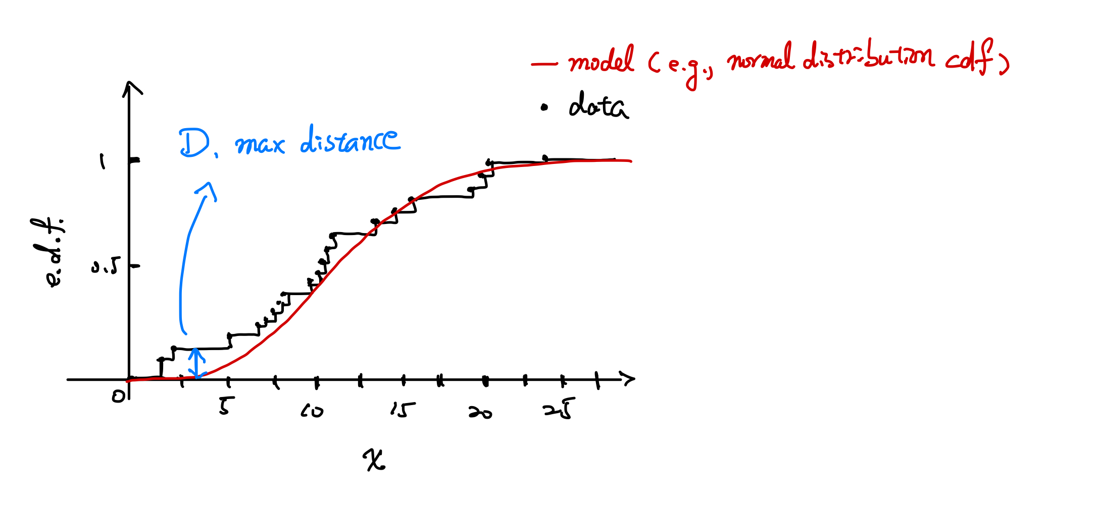
The Empirical Distribution Function (EDF) is a discrete version of the Cumulative Distribution Function (CDF). It is defined as: $$ F_n(x) = \frac{1}{n} \sum_{i=1}^n I[x_i \leq x] $$ where $I[\xi]$ is the indicator function, equating to 1 if the condition is true and 0 otherwise. This means each step in the EDF has a height of $\frac{1}{n}$. An example plot of an EDF is shown below.

Kolmogorov-Smirnov Test (KS Test)
The Kolmogorov-Smirnov (KS) Test measures the maximum distance ($D$) between two distribution functions. This can be used to compare an empirical distribution with a theoretical model (one-sample test) or two empirical distributions (two-sample test). If the distributions are identical, $D$ equals zero.
Statistic: $$ D_n = \max_x |F_n(x) - S_n(x)| $$ A table for the critical values of $D_n$ can be found here.
If $D_n$ exceeds the critical value, we can reject the null hypothesis that there is no significant difference between the two distributions.
Cramér-von Mises Statistic (CvM)
The Cramér-von Mises statistic is used to quantify the goodness of fit of an empirical distribution to a theoretical model. It is particularly useful as it considers the squared differences over all points, providing a more sensitive measure to differences in the tails of the distributions.
This statistic assesses the integrated squared distance between the empirical distribution function $F_n(x)$ and the theoretical distribution $S(x)$, weighted by the number of observations $n$.
Anderson-Darling Statistic (AD)
The Anderson-Darling statistic is a modification of the Cramér-von Mises statistic that gives more weight to the tails of the distribution. It is particularly effective in identifying departures from a theoretical distribution in the tails.
This weighted approach makes the AD statistic more sensitive to discrepancies in the distribution’s tails than the CvM statistic.
Both CvM and AD tests are powerful tools for statistical hypothesis testing, especially in scenarios where understanding the tail behavior of distributions is crucial.
Wilcoxon Rank Sum Test
The Wilcoxon Rank Sum Test, also known as the Mann-Whitney Rank Sum test, is designed to assess whether two independent samples come from the same distribution. Here’s how the test statistic is calculated:
- Combine and Rank the Data:
- Combine all observations from both samples into a single dataset.
- Rank all observations from the smallest to largest. Ties are given a rank equal to the average of the ranks they would have otherwise occupied.
- Calculate the Rank Sums:
- Calculate the sum of the ranks for observations from each sample separately. Let $T_1$ be the sum of ranks for the first sample, and $T_2$ for the second sample.
- Compute the Test Statistic:
- The test statistic $U$ is calculated using: $$ U = T_1 - \frac{n_1(n_1+1)}{2} $$ where $n_1$ is the number of observations in the first sample. $U$ can also be computed for the second sample, and the smaller of the two $U$ values is often used as the test statistic.
- Determine the Significance:
- The significance of the observed $T_1$ value is determined by comparing it to values in a reference distribution, which approximates a normal distribution under the null hypothesis when the sample sizes are sufficiently large. The mean and standard deviation of $T_1$ are used to compute a z-score: $$ |z| = \left| \frac{T_1 - \text{mean}(T_1)}{\text{std dev}(T_1)} \right| $$ where $\text{mean}(T_1) = \frac{n_1(n_1+n_2+1)}{2}$, and $\text{Var}(T_1) = \frac{n_1 n_2(n_1+n_2+1)}{2}$.
- The p-value is then calculated from the normal distribution.
The Wilcoxon Rank Sum Test does not require the data to follow a specific distribution, making it a robust and widely applicable non-parametric method for comparing two samples.
Kruskal-Wallis Test
The Kruskal-Wallis (KW) test is used to determine if there are statistically significant differences between the distributions of two or more groups of an independent variable. It generalizes the Wilcoxon Rank Sum Test to more than two groups. The null hypothesis assumes that all groups come from identical distributions. The test statistic follows a chi-squared ($\chi^2$) distribution with $k-1$ degrees of freedom, where $k$ is the number of groups.
Comparison of Statistical Distribution Tests
| Test | Key Usage | Data Requirement | Distribution Assumption | Sensitivity |
|---|---|---|---|---|
| KS Test | Comparing a sample with a reference distribution | One or two samples, continuous or ordinal | None | Sensitive to differences in location, scale, and shape |
| CvM Statistic | Testing goodness of fit to a theoretical distribution | One sample, continuous | None | Integrates squared differences; sensitive across entire distribution |
| AD Statistic | Testing goodness of fit with emphasis on tail differences | One sample, continuous | None | Increased weight to tails; highly sensitive to tail discrepancies |
| Wilcoxon Rank Sum | Comparing two independent samples | Two independent samples, ordinal or continuous | None | Sensitive to differences in medians |
| Kruskal-Wallis | Comparing more than two independent samples | Two or more independent samples, ordinal or continuous | None | Generalization of Wilcoxon, sensitive to differences across multiple samples |