Clustering and Classification

Clustering and classification are fundamental techniques in data analysis and machine learning, used to group data points based on similarities and to categorize them into distinct classes.

Hierarchical Clustering

Hierarchical clustering builds nested clusters by progressively merging or splitting them based on the distance between data points or groups. The method relies heavily on the choice of distance calculation:

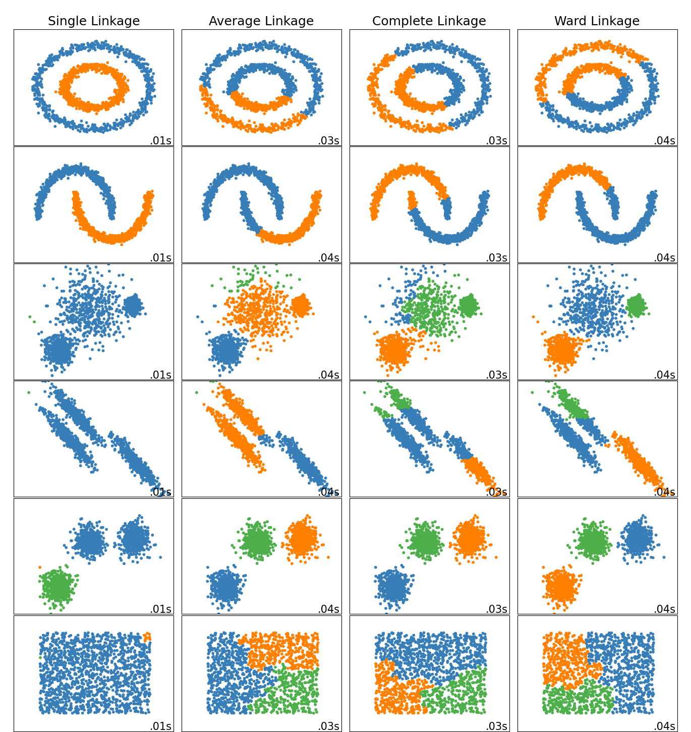
• Single Linkage (Nearest Neighbor): This method, also known as the friend-of-a-friend technique, considers the shortest distance between points in two clusters (see the first plot below). It can result in elongated, “chain-like” clusters that capture local structure but might miss broader data groupings (see the second plot below).
• Complete Linkage: Use the maximum distance between points in two clusters. This method tends to produce more compact and well-separated clusters, reducing the chain effect seen in single linkage.
• Average Linkage: Calculates the average distance between all pairs of points in two clusters. This method provides a balance between the sensitivity of single linkage and the strictness of complete linkage.
• Ward’s Minimum Variance: Minimizes the total within-cluster variance. At each step, the pair of clusters with the minimum increase in total variance are merged. This method tends to create more regular-sized clusters (e.g., spherical or ellipsoidal), which can be advantageous for certain datasets.

(Figure credit: https://www.researchgate.net/figure/The-three-linkage-types-of-hierarchical-clustering-single-link-complete-link-and_fig57_281014334)

Once distances are calculated, the hierarchical clustering algorithm uses these distances to merge or split clusters:

1. Initialization: Start by assigning each data point to its own cluster.
2. Merge Step: At each step, merge the two clusters that are closest together, based on the distance calculation method chosen.
3. Update Distances: Recalculate the distances between the new cluster and each of the old clusters.
4. Repeat: Continue merging clusters until all data points are merged into a single cluster or until a desired number of clusters is reached.

These different linkage criteria can significantly impact the shapes and sizes of the clusters formed. A nice demonstration in various clustering scenarios can be found on the scikit-learn page, also shown below: (Figure credit: https://scikit-learn.org/stable/auto_examples/cluster/plot_linkage_comparison.html#sphx-glr-auto-examples-cluster-plot-linkage-comparison-py)

k-Means Clustering

k-Means clustering partitions the data into $k$ mutually exclusive clusters, and returns the index of the cluster each point belongs to. This method aims to minimize the within-cluster sum of squares.

Density-Based Spatial Clustering of Applications with Noise (DBSCAN)

DBSCAN groups together closely packed points and marks points in low-density regions as outliers. This method does not require specifying the number of clusters a priori, making it suitable for data with irregular or complex structures.

• Parameters:
  • $\mu$: Minimum number of points required to form a dense region.
  • $\varepsilon$: Specifies the “reach”, that is, the distance threshold within which points are considered neighbors.

k-Nearest Neighbor (k-NN)

k-Nearest Neighbors (k-NN) is primarily a classification technique renowned for its simplicity and effectiveness, especially suited for datasets where the decision boundaries between classes are not linear. The k-NN algorithm classifies new data points based on the majority vote of their k nearest neighbors in the feature space.

To apply k-NN effectively, data is typically split into two sets:

• Training Set: This dataset is used to ’train’ or ‘fit’ the model. It includes both the input features and the corresponding classification labels which are known.
• Test Set: This dataset is used solely for testing the performance of the trained model. It helps to evaluate how well the k-NN model generalizes to new, previously unseen data.

Once the model has been trained on the training set, it can be used to predict the class labels of new data in the test set, providing a measure of its classification accuracy.