Kriging

Introduction to Kriging

Kriging is a geostatistical interpolation technique that uses spatial correlation models, such as variograms, to predict values at unsampled locations based on the values at sampled locations. There are several types of Kriging, each with specific assumptions and applications:

• Simple Kriging: Assumes the mean of the random field is known and constant throughout the region of interest.
• Ordinary Kriging: Assumes the mean is unknown but constant within the region of interest and is the most commonly used form as one do not know the mean in real world.

More on Variogram

The semivariance $\gamma(x_1, x_2)$ between two points can be expressed as: $$ \gamma(d) = \frac{1}{2n} \sum_{i=1}^n [z(x_i + d) - z(x_i)]^2 $$ where $n$ is the number of pairs, $d$ is the distance between two points, and $z$ represents the values at the locations. The calculation of $\gamma(d)$ involves several key assumptions:

• Stationary (homogeneous): Assumes that the statistical properties (mean, variance) of the process do not change over space. This implies that the mean and variance are constant throughout the region of interest, and the covariance between any two points depends only on the distance and direction between them, not on their absolute locations.
• Isotropy: Assumes that the statistical properties are the same in all directions. This means that the variogram is a function only of the distance between sample points, not of the direction.

In Kriging, we use $\gamma$ to weight the data for interpolation:

$$\begin{align} \gamma(d) &= \frac{1}{2n} \sum_{i=1}^n [z(x_i + d) - z(x_i)]^2 \\ &= \frac{1}{2} E\left(\left[z(x+d) - z(x)\right]^2\right) \text{(homogeneous assumption)} \\ &= \frac{1}{2} \left\{ E\left[ z^2(x+d) \right] + E\left[ z^2(x) \right] - 2E\left[ z(x+d) z(x) \right]\right\} \\ &= \frac{1}{2} \left\{ 2E\left[ z^2(x) \right] - 2E\left[ z(x+d) z(x) \right]\right\} \text{(homogeneous assumption)} \\ &= \sigma_x^2 + \mu_x^2 - \text{cov}[z(x), z(x+d)] - \mu_x^2 \end{align}$$

where the relationships: $E[x^2] = \sigma_x^2 + [E(x)]^2$ and $\text{cov}[X,Y] = E(XY) - E(X)E(Y)$ were used to get the second to last equation. We have: $$\begin{align} \gamma(d) &= \sigma^2 - \text{cov}[z(x), z(x+d)] \\ &= \sigma^2 - \text{c}(d) \end{align}$$

Therefore, we have the semivariance at distance $d$ is the variance minus the covariance between points at this distance.

Example of Spatial Data and the Kriging Result

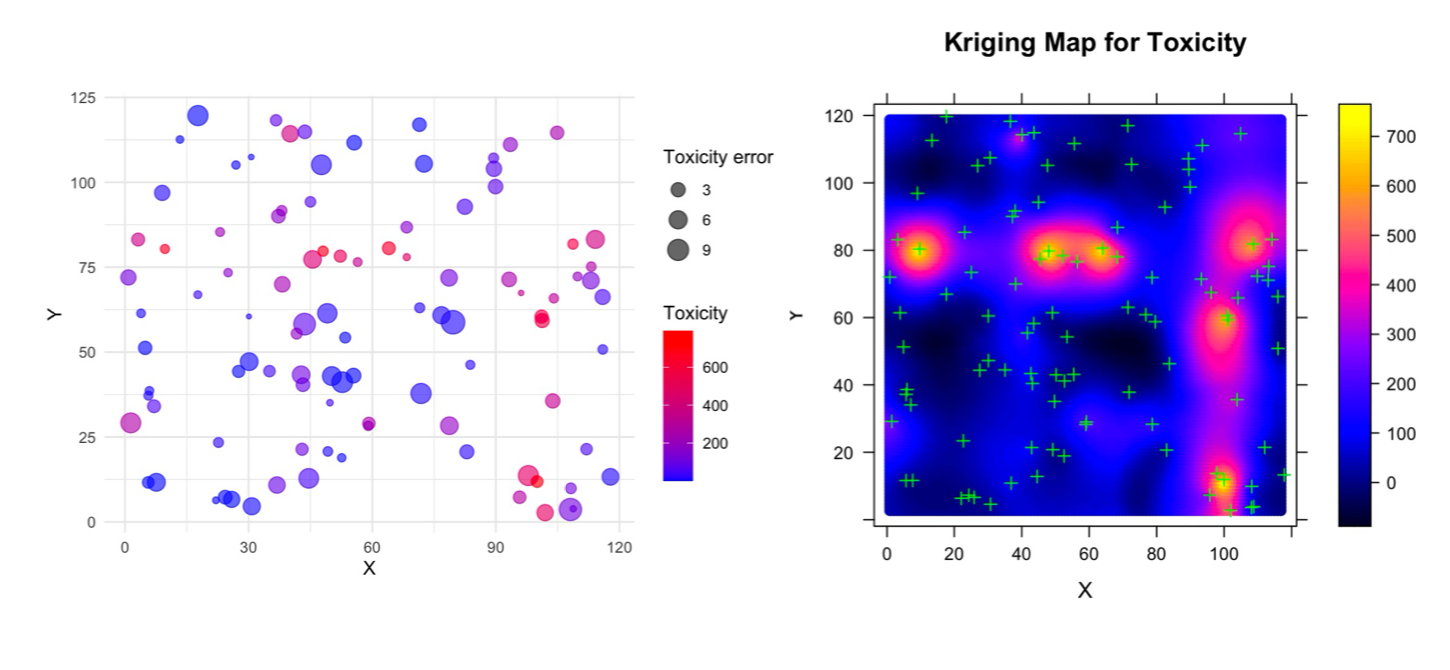
The plots below show an example of spatial data (left) and its associated Kriging map (right). The data used here is the same as in the Variogram page, and the Kriging map uses the variogram model shown on the Variogram page to predict values at unsampled locations. This example demonstrates how Kriging utilizes the spatial structure of the data, as defined by the variogram, to provide a statistically optimal interpolation.

Figure data credit: Charles M Pacheco

Example R Code for the Kriging

# Fit a variogram model
vgm_model <- vgm(psill = max(variogram_tox$gamma), 
       model = "Sph", range = 30)
       
x.range <- range(df_2$x)
y.range <- range(df_2$y)

grid.points <- expand.grid(
       x = seq(from = x.range[1], to = x.range[2], by = 1),
       y = seq(from = y.range[1], to = y.range[2], by = 1))

# Convert to SpatialPoints
grid <- SpatialPoints(grid.points)

# Perform ordinary kriging
kriged <- krige(toxicity ~ 1, df_2, model = vgm_model, newdata = grid)

options(repr.plot.width=5, repr.plot.height=5, repr.plot.res=200)
# Create a map with overlay contours
spplot(kriged, "var1.pred", main = "Kriging Map for Toxicity", 
       xlab = "X", ylab = "Y",
       sp.layout = list("sp.points", df_2, col = "green"),
       colorkey = TRUE,
       scales = list(draw = TRUE))